The Quixotic Quest: Why searching for a de facto species
sensitivity distribution is futile and unnecessary

David R. Fox^a,b,*, Rebecca Fisher^c, Joe Thorley^d

^a Environmetrics Australia, P.O. Box 7117, Beaumaris, Victoria, Australia 3193 

^b Department of Infrastructure Engineering, University of Melbourne, Parkville, Victoria, Australia 3010

^c Australian Institute of Marine Science,

^d Poisson Consulting, Nelson, British Columbia, Canada

INTRODUCTION

Contrary to the recent claim that the problem of identifying a ‘default’ probability model for the species sensitivity distribution (SSD) has received limited attention (Yanagihara et al. 2024), this is an issue that has been tackled by several authors including (Beaudouin and Péry 2013, Fox et al. 2021, Fox 2016, Wheeler et al. 2002, Xu et al. 2015). While well-intentioned, such efforts are ultimately fraught and unlikely to yield conclusions and recommendations that are (a) consistent; and (b) of practical value. This is primarily by virtue of the following:

1. Recommendations arising from the analysis of empirical or simulated data sets cannot be easily generalized. This is particularly true for empirical data sets for which the ‘true’ response-generating model is unknown and unknowable. This limitation was acknowledged by Yanagihara et al. 2024 who stated “making rigorous comparisons is difficult because of variations in the sets of statistical distributions examined and the methodologies used for selecting the ‘best’ model”.
2.  Omnibus recommendations are heavily dependent on the nuances of the data sets used, the selection of statistical models, the modes of statistical analysis (including narrowing the scope of analysis), the treatment of outliers, violation of assumptions and other aberrations such as multimodality.
3.  The well-documented fact that there is no theoretical basis to guide the choice of statistical distribution for the underlying SSD (Fox et al. 2021, Fox 2016).
4.  Absence of motive. There is no need to identify a single ‘best’ candidate probability model for the SSD.

On this last point, we note that recent advances in SSD modelling and inference have reduced, if not eliminated the need to choose a single distribution. Over the past 5 years we have been jointly funded by the Australian, New Zealand, and Canadian governments to undertake a ‘deep dive’ into the mathematical, statistical, and computational underpinnings of statistical model averaging in the context of fitting SSDs and using these to obtain robust, statistically defensible, and scientifically credible estimates of protective concentrations (PC_x) and fractions affected (FA). Our recent reports <here> detail the results of exhaustive testing and analysis as well as providing recommendations on the adoption of our companion R package ssdtools and on-line implementation, shiny(ssdtools) has been accepted by all three jurisdictions. It is expected that ssdtools will soon be endorsed as the de facto software tool for use by researchers, consultants, and analysts in those jurisdictions. For these reasons, we disagree with the assertion by Yanagihara et al. (2024) that “the adoption of the model averaging for SSD estimation in many jurisdictions worldwide is not yet common”. In addition to Australia, New Zealand, and Canada, the United States EPA has a software tool (ssdtoolbox) which can fit model-averaged SSDs <here>. While we are unaware of any specific European Union guidance on the use of model-averaged SSDs, the concept itself is routinely used in the related activity of concentration-response (CR) modelling in which the benchmark dose (BMD) is determined using a model-averaged fit to CR data <here>.

THE QUIXOTIC QUEST

In the Yanagihara et al. (2024) study, the lognormal distribution was effectively held up as the ‘gold standard’ against which each of only three other distributions were required to demonstrate overwhelming superiority. That Yanagihara et al. (2024) confirmed the role of the lognormal distribution despite the superiority of the Weibull distribution 25% more often than the lognormal for acute data and 30% more often than lognormal for chronic data is suggestive of research confirmation bias (Casad and Luebering). A partial explanation for this is revealed by the Cullen-Frey plot of the data used by Yanagihara et al. (2024) (Figure 1) which, interestingly was not plotted by Yanagihara et al. (2024) despite them having having used the R package e1071 to calculate the kurtosis skewness of their toxicity data. The obvious feature of Figure 1 is the fact that the empirical skewness-kurtosis values closely follow the contour of the Burr (k=0.001) distribution and are uniformly ‘closer’ to the Weibull distribution than the lognormal distribution.

Figure 1. Cullen-Frey plot showing contours for selected theoretical distributions (solid lines) and empirical skewness-kutosis pairs for the
Yanagihara et al. (2024) acute and chronic data (solid red circles).

In 2 above we highlighted the issue of studies having a narrow focus or restricted scope. We are perplexed as to why Yanagihara et al. (2024) dismissed model-averaging as being “beyond the scope of this study” when they used the ssd_hc() function in our model-averaging software (ssdtools) to estimate separate HC₅ values for each of the four distributions considered.  The help on function ssd_hc() states that it “calculates concentration(s) with bootstrap confidence intervals that protect specified proportion(s) of species for individual or model-averaged distributions using parametric or non-parametric bootstrapping” (emphasis added). Indeed, one of the default settings for ssd_hc()is multi_est = TRUE which ensures that HC values are estimated using a model-averaged SSD. So, it would appear that the default model-averaging was deselected on the basis that it was out-of-scope.

Further, in 3 we highlight the fact that there is no theoretical basis for selection of a single distribution for SSD modelling. Indeed, across the many datasets examined in The Yanagihara et al. there are multiple datasets that are best represented by each of the six univariate distributions in ssdtools (Figure 2). Notably, the log Gumbel and gamma, both of which were excluded from the original analysis of Yanagihara et al., frequently represented the best fitting distribution across the many chronic and acute datasets (Figure 2).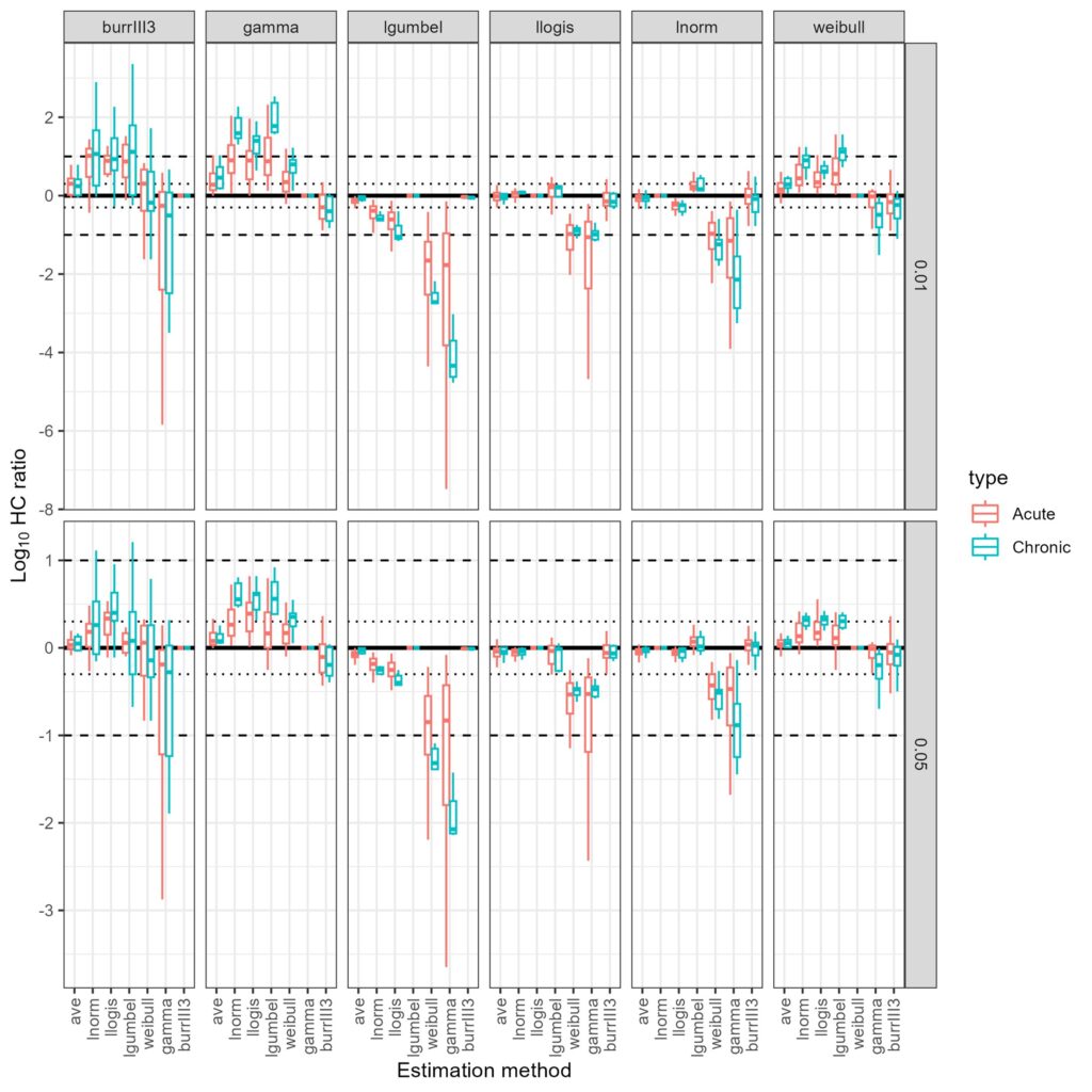

Figure 2. Log10 HC ratio calculated for each dataset as the ratio of the HC value estimated from the distribution with the highest AICc based model
weight against the HC value estimated from each of the candidate univariate distributions. Also include are the model averaged HC
estimates provided by ssdtools as default. Ratios for both HC1 and HC5 values are shown, for Acute and Chronic datasets.

Finally, in 4 we identified the absence of motive. The Yanagihara et al. (2024) study provides evidence of both.

A RE-EVALUATION

We re-analysed the data considered in Yanagihara et al. (2024) to assess the validity of their general conclusions and provide a more complete understanding of the potential value provided by model averaging. In our re-analysis we included six of the available univariate distributions in ssdtools, and also expanded the analysis to include both the HC1 as well as the HC5. Further, rather than considering the lognormal distribution as the default “baseline” instead we calculated log ratios for HC values, assuming the distribution with the highest AICc based model weight as the baseline.

When Log10 HC ratios are calculated using the best fitting distribution as the baseline we found substantial variation in HC estimates across the six candidate distributions. In particular, when the best fitting distribution is the log Gumbel, HC estimates obtained using a Weibull and gamma distributions (which have highest deviation in tail behaviour from the log Gumbel) yielded much higher HC values, with Log10 ratio values below -2 for the HC5 (Figure 2). The outcome is substantially worse when the HC1 is considered, with ratios often below -2 for datasets best fit using a Burr III, log Gumbel, log Logistic even the log normal distribution (Figure 2).

Log10 HC ratios for both the HC1 and HC5 estimates based on the default model averaging approach of ssdtools were all very close to the expected value of 0 for all baseline distributions (Figure 2), suggesting model averaging effectively resolves the dilemma of attempting to select a single best-fitting distribution (Figure 2).

CONCLUSIONS AND RECOMMENDATIONS

The Yanagihara et al. (2024) study is the latest output from the ‘cottage industry’ dedicated to answering the unanswerable: what is the best distribution to use for an SSD?

Unlike other branches of physical science where the development of ‘rules’ or formulae is predicated on, if not governed by, solid theory (e.g. E = Mc² ; F=MA ; Temp = e^–kt etc.) species sensitivity modelling is not so fortunate – there is absolutely no theory in ecotoxicology which provides even the feintest guidance on the appropriate form of the SSD (other than it be a probability model on ℝ⁺). The sooner there is universal acceptance of this fact, the sooner the discipline can move on to more productive avenues of investigation such as the best way of identifying and dealing with bi and multimodality and how to deal with mixtures of chemicals.

For these reasons, we make a simple and impassioned plea to the ecotox. research community: stop the endless cycle of comparative studies based on a handful of small real data sets or large samples from simulations under a small set of prescribed conditions to try to make general recommendations about the ‘best’ distributional form for an SSD. It is the ultimate quixotic quest.

REFERENCES

Beaudouin, R., Péry, A.R.R. 2013. Comparison of Species Sensitivity Distributions based on Population or individual endpoints. Environ. Toxicol. Chem. 32, 1173-1177.

Casad, Bettina J. and Luebering, J.E.. “confirmation bias”. Encyclopedia Britannica, 18 Jun. 2024, https://www.britannica.com/science/confirmation-bias. Accessed 30 July 2024.

Fox, DR.  2016.  Contemporary Methods for Statistical Design and Analysis, in Marine Ecotoxicology. Editor(s): Julián Blasco, Peter M. Chapman, Olivia Campana, Miriam Hampel,
Academic Press, pp 35-70, https://doi.org/10.1016/B978-0-12-803371-5.00002-3.

Fox, D.R., van Dam, R.A., Fisher, R., Batley, G.E., Tillmanns, A.R., Thorley, J., Schwarz, C.J., Spry, D.J., McTavish, K., 2021. Recent developments in species sensitivity distribution modeling. Environ. Toxicol. Chem. 40, 293–308.

Wheeler, J.R. Grist, E.P.M., Leung, K.M.Y., Morritt, D., Crane, M. 2002. Species sensitivity distributions: data and model choice. Marine Pollution Bulletin, 45, 192-202. DOI10.1016/S0025-326X(01)00327-7.

Xu, Li, YL, Wang, Y , He, W , Kong, XZ , Qin, N , Liu, WX , Wu, WJ , Jorgensen, SE. 2015.  Key issues for the development and application of the species sensitivity distribution (SSD) model for ecological risk assessment. Ecological indicators, 54, 227-237.